Estimating peak gas demand in European Member States

• Joint Research Centre, European Commission, Petten, The Netherlands [anca.costescu@ec.europa.eu]

• Joint Research Centre, European Commission, Petten, The Netherlands [ricardo.bolado-lavin@ec.europa.eu]

Keywords: Peak gas demand – Extreme value theory

1 Introduction

The European Union’s Regulation (EU) 2017/1938 outlines measures to ensure the security of gas supply across member states. According to this regulation, each member state must implement necessary measures to guarantee that, in the event of a disruption to the single largest gas infrastructure, the remaining infrastructure can meet the total gas demand of the affected area on a day of exceptionally high gas demand, which is statistically expected to occur once every 20 years (1-in-20).

The national Transmission System Operators (TSOs) have been collecting daily gas demand data, and since 2015 all those data are regrouped in ENaGaD database (Zaccarelli et al. [2021]). Meteorological institutions across member states have been collecting temperature data since quite a long time. Here, we chose to use the average (per country) daily temperatures (in ${}^{\circ }$C) since 1991, from https://agri4cast.jrc.ec.europa.eu/.

Notably, during the winter period, when high gas demand typically occurs, the relationship between gas demand and temperature can be accurately modeled using linear regression.

To estimate the extremely high (or peak) gas demand with a statistical probability of 1-in-20, we propose here a three-step methodology:

1. Apply the Extreme Value Theory (Coles et al. [2001]), specifically the generalized extreme value (GEV) distribution for block maxima, to estimate the 1-in-20 extreme temperature.

2. Develop a linear regression model that links gas demand to temperature, as well as other relevant explanatory variables.

3. Use this model to estimate the gas demand corresponding to the 1-in-20 temperatures in the first step, thereby determining the peak gas demand.

This methodology is illustrated using data from Germany.

2 Estimation of the 1-in-20 temperature

The general form of a GEV distribution is (see Coles et al. [2001]):

$$G(z)=\exp \{-{[1+\xi (\frac{z-\mu }{\sigma })]}^{-1/\xi }\}$$

such that $1+\xi (\frac{z-\mu }{\sigma })>0$. The parameters $\mu \in \mathrm{I}\mathrm{R}$, $\sigma >0$, $\xi \in \mathrm{I}\mathrm{R}$ are the location, scale and shape parameters respectively. The notation used is $Z\sim GEV(\mu ,\sigma ,\xi )$. The parameters are estimated by maximum likelihood.

In order to fit a GEV, one of the main assumptions is that the process (i.e. the time series) is stationary. Non-stationary processes have characteristics that change systematically through time. In the context of meteorological processes, non-stationarity may be present in the form of trends, possibly due to long-term climate changes. A suitable model for a process showing a linear trend is $Z_t\sim GEV(\mu (t),\sigma ,\xi )$, with $\mu (t)={\beta }_0+{\beta }_{1}t$. A statistical test, based on the difference of the log likelihoods for the stationary and the non-stationary models, is performed to check whether the non-stationary model is significant compared to the stationary one.

A return level $z_p$ associated to a return period of $1/p$ is obtained by solving the equation $G(z_p)=1-p$. The solution is

$$z_p=\mu -\frac{\sigma }{\xi }[1-{(-\log (1-p))}^{-\xi }]$$

where $\mu$ can be a function of time, $\mu =\mu (t)$. For a 20-years return period, the probability $p$ is equal to $1/20=0.05$. A confidence interval (or a confidence band, for time dependence) is also inferred for the return level.

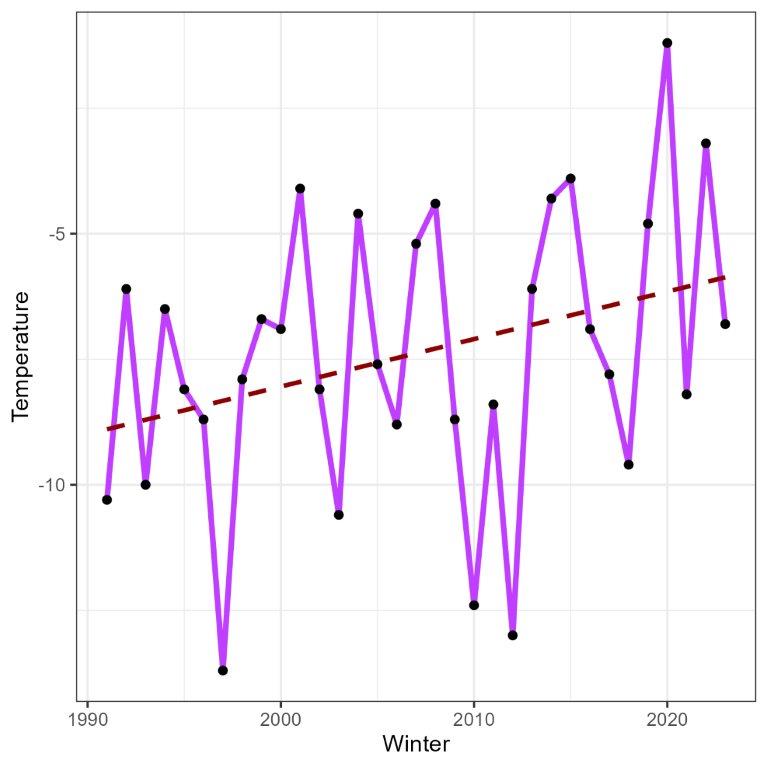
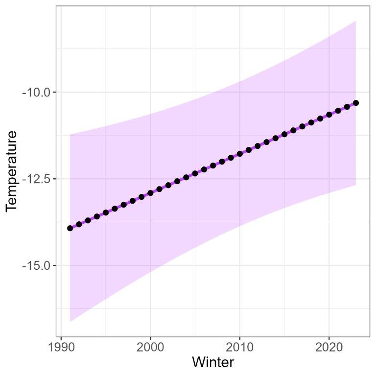
We consider the daily average temperatures in Germany for the period 01/01/1991 – 31/12/2022. We define a block as the period between December of year $t$ and February of year $t+1$. In this way, the block represents the peak period of a gas year. Within each block, the minimum temperature is selected, resulting in a time series with 33 values. Those 33 values are used to fit the GEV distribution and are shown in Figure 1 (left). The estimate of the 1-in-20 extreme temperature together with its 95% confidence band is shown in Figure 1 (right). Calculations have been carried out using the package extReme(see Gilleland and Katz [2016]) of the statistical software R.

Figure 1: Minimum temperature per winter season (left) and estimation of the 1-in-20 per winter season and its 95% confidence band (right)

3 Model demand temperature

The final linear regression model for the gas demand has, beside the average temperature of the day, the following explanatory variables: a dummy variable for the day of the week (either normal weekday or week-end), a dummy variable for the validity of the Regulation (EU) 2022/1369 on reducing gas demand in the EU by 15%, a dummy variable for the month (December, January or February) and Fourier terms for the Julian day. The adjusted $R^2$ of the model is 0.867, and the coefficients are in Table 1.

Table 1: Linear regression model

Predictor	Est.	p - value	significance
(Intercept)	-2073	0.001	$**$
temperature	-159		$***$
weekWeekend1	-346		$***$
reduction1	-410		$***$
month2	-224	$2e-06$	$***$
month12	-240	$3e-07$	$***$
$\cos (2\pi$ day/365)	9893		$***$
$\cos (4\pi$ day/365)	-3418		$***$
$\sin (4\pi$ day/365)	-160	0.0002	$***$

4 Estimation of the peak demand

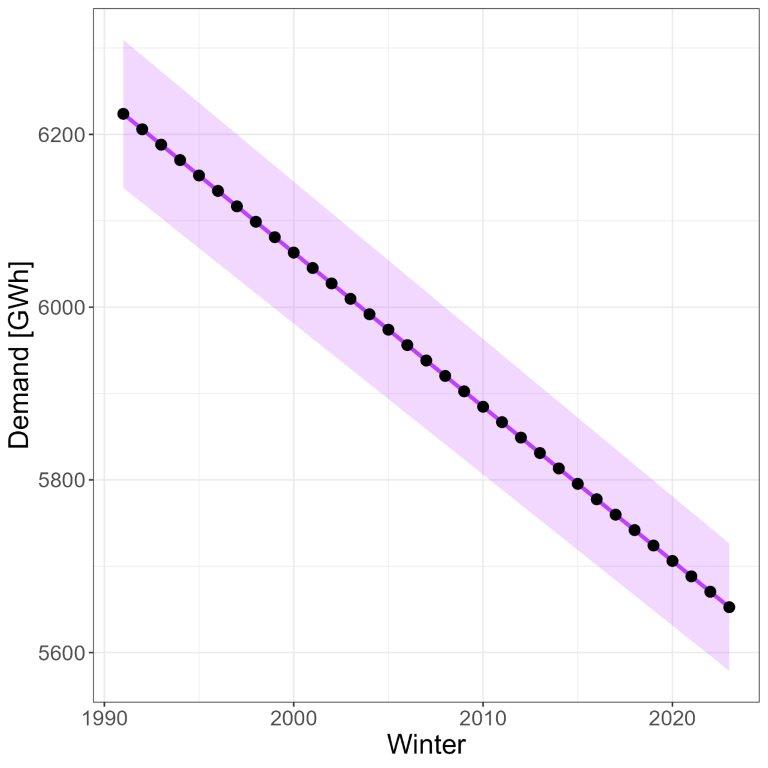
We used this model to estimate the gas demand corresponding to the 1-in-20 extreme temperatures calculated in the first step, thereby determining the peak gas demand. In Figure 2 the peak demand is estimated assuming that we are on January 15, a normal week day, and that the demand reduction still applies. This estimate of the peak demand is in the range 5668 GWh – 6241 GWh. For comparison, ENTSO-G considers in it’s winter outlook (see von der Grün et al. [2024]) a peak demand for cold winter of around 6700 GWh.

Figure 2: Germany. The peak gas demand 1-in-20 with 95% confidence band

References

- Coles et al. [2001] Stuart Coles, Joanna Bawa, Lesley Trenner, and Pat Dorazio. An introduction to statistical modeling of extreme values, volume 208. Springer, 2001.
- Gilleland and Katz [2016] Eric Gilleland and Richard W Katz. extremes 2.0: an extreme value analysis package in r. Journal of Statistical Software, 72:1–39, 2016.
- von der Grün et al. [2024] Thilo von der Grün, Kacper Zeromski, Arturo de Onis, and Diana Fathelbajanova. Winter supply outlook 2024/25. ENTSOG AISBL: 1000 Brussels, Belgium, 2024.
- Zaccarelli et al. [2021] Nicola Zaccarelli, Sergio Giaccaria, Maksims Feofilovs, and R Bolado-Lavín. The european natural gas demand database (ENaGaD). Luxembourg: Publications Office of the European Union. doi, 10:497677, 2021.